Optimizing Python (Using Built-Ins)

Introduction

First and foremost when we are trying to make our Python code run faster, we should focus on taking advantage of code that is already written for us. The base Python language has a wide variety of built-in functions, ranging from determining an absolute value with the abs() function to iterating through several lists at the same time with the zip() function. Generally speaking, these built-in functions are implemented at a lower level in compiled C code, and are significantly faster than doing the equivalent task ourselves in Python.

First example: finding min / max

A frequent task faced by programmers is to find the minimum and maximum elements in a list. And, it is easy enough to write Python code to complete the task, as shown here in Sample 1.

1
2
3
4
5
6
7
8
9
# Sample 1: finding min / max of a list, native Python code
# assume values is a list containing floats in [0, 1)
minimum = 2.0
maximum = -2.0
for v in values:
    if v < minimum:
        minimum = v
    if v > maximum:
        maximum = v 

Sample 1 starts by initializing the variables minimum and maximum to values that are, respectively, larger than or smaller than any element in the list could be. Then, the code uses a for loop to iterate through all of the values in the values list. For each value, we use an if statement to see if it is smaller than the current value for minimum. If that is the case, we have a new minimum value, so we update the value of minimum. A similar if statement keeps track of the current maximum value in the variable maximum. After the loop is complete, we have examined each value in the list, and therefore the values of minimum and maximum will be correct.

As simple as this code is, Python has two built-in functions, min() and max(), that perform the same function. Sample 2 shows code that finds our minimum and maximum values with these built-in functions instead of our “homemade” solution in Sample 1.

1
2
3
# Sample 2: finding min / max of a list, with built-ins
mininum = min(values)
maximum = max(values)

The first, most obvious benefit of using the built-in max() and min() functions is that doing so requires less typing on our part, while the code is still straightforward and easy-to-read.

The bigger benefit, from our point of view here, is that Sample 2 is significantly faster in execution than Sample 1, as shown in this plot:

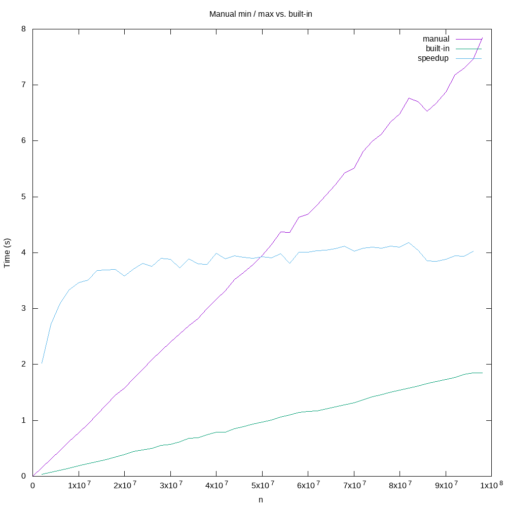
We can see that the speedup caused by using the built-in min() and max() functions is roughly four, meaning that Sample 2 is approximately four times faster than the native Python version shown in Sample 1. To make this even more interesting, consider that the loop in Sample 1 goes through the list only one time, while the built-in functions in Sample 2 iterate through the list twice: once for min() and once again for max(). The low-level code for these built-in functions is fast enough that iterating through the list twice to accomplish the task is still four times faster than the native Python version.

So, it makes good sense to keep the 70 or so Python built-in functions close at hand, mentally, when we write code. If we can utilize these functions in our code, not only will we have less code to write, our code will almost certainly be faster if we use built-ins than if we accomplish the same task with native Python code.

Tip: Whenever possible, use built-in Python functions instead of writing “native” Python code.

Second example: matrix multiplication

Python is known for its ease of use and for the numerous modules and libraries that can be imported for just about any problem domain, as this tongue-in-cheek xkcd comic illustrates:

The standard distribution of Python alone contains over 200 modules, and there are something like 137,000 other libraries available to be installed and used by Python programmers. We cannot vouch for the quality of all 137,000 libraries, but the odds are pretty good that there is a module already written to do some or all of the problem you are trying to solve. Many of these modules have the extra benefit of being implemented in low-level C code, meaning that they are very fast in their operation, just as we saw for the built-in min() and max() functions.

Here we will consider a somewhat extreme example, while also taking the opportunity to introduce the widely used NumPy scientific computing package. The problem we will solve is matrix multiplication, which is a very common task in scientific computing.

If matrix A has m rows and n columns,

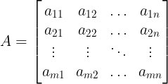
and matrix B has n rows and p columns,

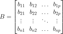
Then the matrix product C = AB is a new matrix of m rows and p columns where for i = 1..m and j = 1..n,

C as a whole looks like this:

This is a very common computation, and relatively straightforward to implement, as shown in the native Python code in Sample 3. Here, to simplify things slightly, we are considering the multiplication of two square, n * n matrices. A and B have already been constructed and filled with random values, and space for the result matrix C has already been allocated. All three matrices are NumPy arrays, rather than Python lists of lists.

1
2
3
4
5
6
# Sample 3: matrix multiplication in native Python

for i in range(n):
    for j in range(n):
        for k in range(n):
            Cn[i][j] += A[i][k] * B[k][j]

If you have studied computer science, particularly in the analysis of algorithms area, the thrice-nested loops in Sample 3 probably give you pause. Since each loop iterates n times, the overall time complexity of this algorithm is on the order of n³, which is not good. Computationally, matrix multiplication is expensive, and running the code from Sample 3 bears this out. On our test system, multiplying two 1000 by 1000 matrices took, on average, approximately 875 seconds to complete.

We cannot do much to decrease the n³ time complexity of matrix multiplication, but we can execute our matrix multiplication using the highly optimized code provided by the NumPy library. Sample 4 performs the same multiplication using the NumPy matmul() function.

1
2
3
# Sample 4 -- matrix multiplication using NumPy

Cny = np.matmul(A, B)

Again, the first thing that jumps out at a reader of the code is that it is certainly much shorter and simpler than the native Python code above. And, if we are honest, the experts that support NumPy are probably less likely to introduce errors into their code than we would be if we were forced to come up with Sample 3 on our own.

The real difference between Sample 3 and Sample 4 becomes apparent when we compare the run times. Whereas the native Python code took 875 seconds to multiply two 1000 by 1000 matrices, the NumPy equivalent took around 1.39 seconds. The run times for a variety of matrix sizes from 100 to 1000 is shown in this plot:

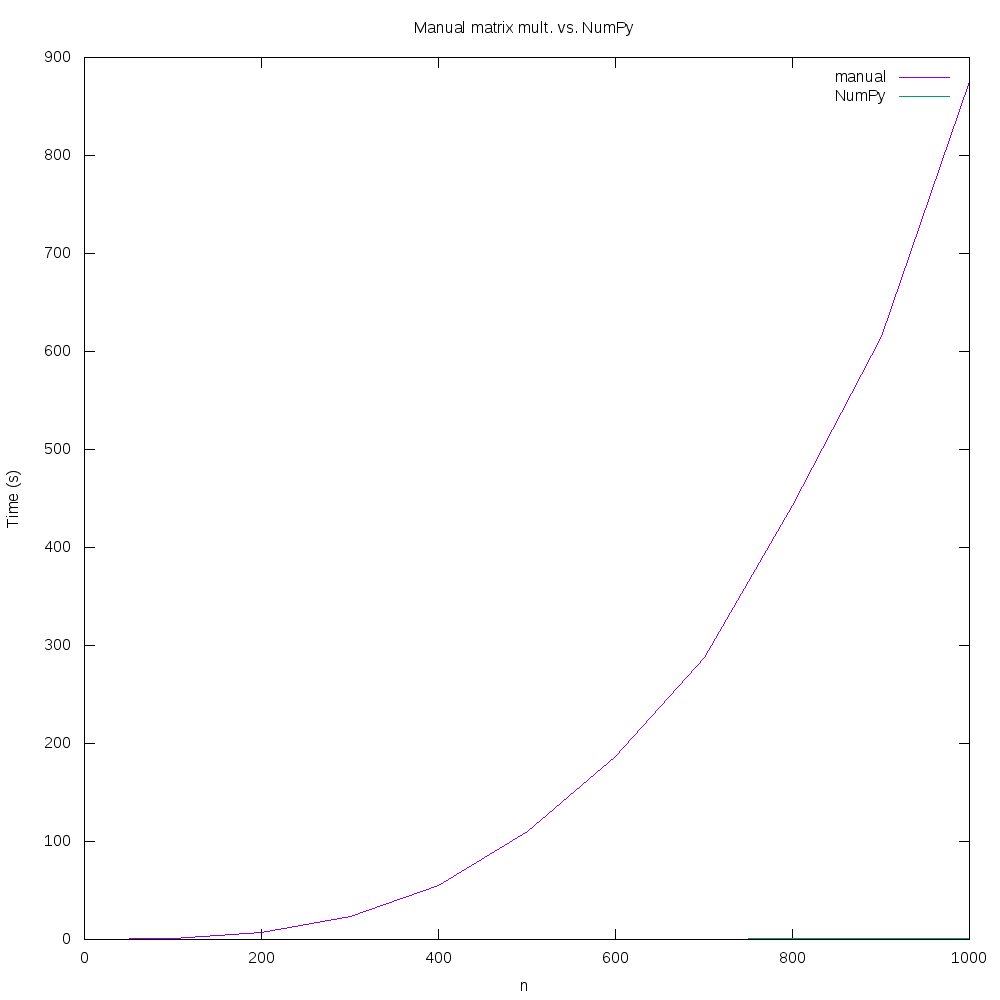
If you look very closely at the plot, you can just barely see the curve representing matrix multiplication with NumPy – the native Python version takes so much more time that the NumPy line barely registers!

We did not draw the speedup line on the previous plot, but here it is on its own:

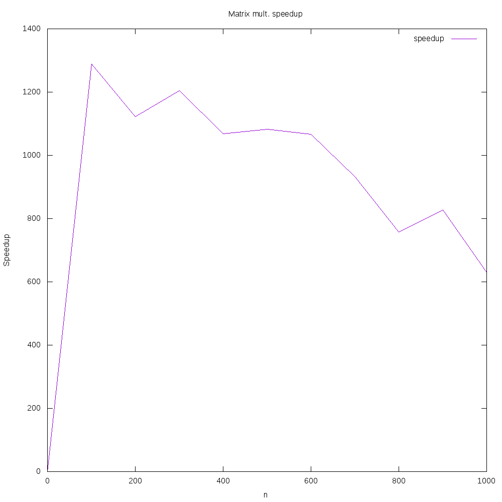
We can see that the speedup is more variable than we have seen previously, but it seems that a speedup on the order of 1000 is reasonable to expect for this code! Accordingly, we should try to use well-tested, well-optimized code in Python libraries when possible.

Tip: Whenever possible, use well-tested, well-documented Python libraries instead of writing “native” Python code.

Exercise 1

Another useful built-in functin in Python is sum(), which can be used to find the sum of the numbers in a list. Finish the code below to calculate the sum of a randomly-populated list using a native Python approach, and then again via the sum() function. The code is instrumented via the timeit module to print out the time taken by each approach, and it also verifies that the two answers received are the same. Once you have written each version, feel free to vary the value of n to see how much time each version takes as the size of the list gets larger and larger.

1
2
3
4
5
6
7
8
9
10
11
12
13
14
15
16
17
18
19
20
21
22
23
24
25
26
27
28
29
30
31
32
33
34
35
36
37
38
# Exercise 1 - summing values

from timeit import default_timer as timer
import random

# list size
n = 100000

# create randomly-populated list
values = [random.randrange(1000) for i in range(n)]

# part 1: write native Python to sum the list,
# using the accumulator pattern; store the sum
# in the variable named nativeSum
nativeStart = timer()

nativeSum = 0
# your code here


nativeStop = timer()

# part 2: find sum via built-in; store the sum
# in the variable named biSum
biStart = timer()

biSum = 0
# your code here

biStop = timer()

print('Native time elapsed:', nativeStop - nativeStart)
print('Built-in time elapsed:', biStart - biStop)

if nativeSum == biSum:
    print('Sums are equal')
else:
    print('SUMS WERE NOT THE SAME')

Exercise 2

Computer images are often stored in 24-bit, Red/Green/Blue (RGB) format, where each pixel is a triple of numbers, each in the closed range [0, 255], representing the relative intensity of the red, green, and blue colors for the pixel. For example, a triple (255, 0, 0) is red, because it has full intensity in the red channel and none in the green or blue channels. Similarly, (0, 255, 0) is pure green and (0, 0, 255) is pure blue. In this color model, (255, 255, 255) represents white and (0, 0, 0) represents black.

This is not the only way to specify RGB values, however. Often, when we perform image processing, we would prefer to indicate the intensity of each channel with a floating-point number in [0, 1]. Representing images this way allows us to perform computations on them in a more numerically stable way.

The code below loads a color image of some Maize seedlings from the Web into a 3-dimensional NumPy array named image.

1
2
3
4
5
6
7
!git clone https://github.com/mmeysenburg/divasii-imgs.git

import skimage.io
import numpy as np

# loads the image
image = skimage.io.imread('divasii-imgs/maize.png')

The first layer of the array represents the red channel, while the second is the green channel, and the third layer is the blue channel. Each value is an integer in [0, 255]. The image is 800 pixels wide by 800 pixels high.

Converting the values in the image to the range [0, 1] would not be too hard to do. We would have three nested loops, similar to the native matrix multiplication code we had above in Sample 3, perhaps something like this:

1
2
3
4
for i in range(image.shape[0]):
  for j in range(image.shape[1]):
    for k in range(image.shape[2]):
      newImage[i][j][k] = image[i][j][k] / 255.0

Given our experience with the natively-coded matrix multiplication code above, we would expect that this natively-coded code would be unacceptably slow. That expectation is correct; on our test system, converting the pixels in this way took nearly 4 seconds.

But, we can take advantage of the capabilities of the NumPy library to perform the same task more quickly, and with only one line of code. Do a little online research to see how to divide all of the elements of a NumPy array by a scalar value, and then complete the code below by finishing the indicated line.

1
2
3
4
5
6
7
8
9
10
11
12
13
14
15
import skimage.io
import numpy as np

# loads the image
image = skimage.io.imread('divasii-imgs/maize.png')
print('values in image:')
print(image)

# convert the image's pixels by dividing each
# value by 255; store in variable named
# newImage
newImage = # finish code here

print('values in new image:')
print(newImage)

Speedup

We refer to speedup as a way to compare our optimized code with its original, slower counterpart. Speedup is a measure of how well we have improved the runtime of our code. If T₀ is the time taken by the original code, and T₁ is the time taken by the improved code, then speedup is defined as

A speedup of 2 would mean that our optimized code is twice as fast as the original, while any value under 1 would mean that we actually made our code slower!

All performance figures on this page were obtained on a Windows 10 PC with an Intel® Core™ i5-9600K CPU @ 3.70GHz and 32GB of RAM, in Python 3.6.9 running in an Ubuntu Windows Subsystem for Linux environment.

Next lesson

The next lesson in the workshop is about List Comprehension